Efficient Routing on a Scale: Winning Solution of the Machine Learning Prague 2021 Hackathon

This post is a walkthrough of the winning solution for the ML Prague 2021 Hackathon problem that my teammate Michał and I came up with.

We were given anonymized data containing approximately 524k Czech policyholders, 44k clinic departments of 273 different types, and 332 ambulance stations. We were tasked with assigning each of the policyholders to the closest of each of the 273 clinics, in addition to the nearest ambulance station. The closest clinics and ambulance stations were supposed to have been picked by the driving distance. To help us with the routing, we were given $200USD in MS Azure credit, which was enough to make 40k routing requests (or 400k if we were willing to go under the 50 queries per second limit). This amount is nowhere near the one required for a brute-force solution, not to mention that it would take a while. We had five days to come up with the solution. On top of that, we were tasked to present our results using SAS Visual Analytics on SAS Vija.

If you prefer video to text, here is our presentation for the conference featuring the dashboard:

The video is denser and less detailed compared to this article.

Before we dive into the code, let’s go over the solution’s summary.

We’ve noticed that 5,827 of 43,908 clinics lacked data essential for the task: type and department_id. Online research failed to turn up a way to fill in the data, so we dropped the clinics that didn’t have these two fields filled in.

Since ambulance stations and clinics had the same data structure, we introduced a new, special type, 'AST', to identify ambulance stations and concatenated two tables into an “organizations” table.

Then, we’ve created a parent_orgs table that grouped organizations by their geolocation, preserving pairings between type and department_id, and thus, giving us a list of 10,797 unique geopoints we had to match users with.

The straightforward approach was to iterate over all users to find the closest organizations by computing driving distances between a user and the organizations, which were sorted by straight line distances, stopping when the straight line distance to the next candidate is larger than the driving distance to the best candidate.

But this approach proved inefficient even taking the sorting optimization into account; in a second-best case scenario, we had to compute 524102*274 routes. The actual best-case scenario number would be lower because a lot of department_ids share the same coordinate.

Instead, we decided to cluster users, compute driving distances to the centroids of the clusters, and approximate actual driving distances and times for each user based on the relation of the direct_distance(user, organization) / direct_distance(cluster_centroid, organization). The algorithm isn’t perfect but gives us a very close approximation and can be computed in a reasonable time.

We clustered users within areas with a max radius of 500m using the combination of village+village_part to speed up clustering and to limit clusters to a single village_part. This provided us with 47,199 clusters, resulting in much more requests than we were comfortable issuing to MS Azure, considering the provided credit amount. Still, we didn’t want to sacrifice precision, so we set up a local OSRM server and used it to compute driving distances.

For direct distance computation, we used the haversine distance instead of the Vincenty, despite the former being less precise for geodesic computations because we could compute the haversine distance much faster. The error margin it introduces is not significant on the scale that we worked with, and both these distances provide optimistic approximations of the driving distance.

We also noticed that there are many deparment_ids of the same type, sharing the exact location. In these cases, we randomly distributed the corresponding users among them to spread the load between departments.

Alternatively, we could’ve used the fact that some people live on the same street to approximate driving distances, but we believe that small clusters approximate actual distances better.

Possible future improvements:

Fill in missing specialty_id and department_id.
Reduce the cluster radius further, allow for more compute time, and re-compute distances with a smaller error margin.
Consider the distance between an ambulance station and a clinic when assigning an ambulance station to a clinic⇔user/cluster pair and choose an ambulance station closer to the clinic if there are multiple stations available within a similarly close distance to the user/cluster, so that the ambulance car can return to the station ASAP.

Now, let’s dive into the code. The code is in Python and is meant to be executed in a Jupyter Notebook.

According to the task, the output CSV should contain a row for each of the policyholder⇔clinic department pair in the following format:

OUTPUT_COLUMNS = [
    'policyholder_num',
    'contractual_specialty_id',  # clinic department type
    'pzs_department_id',  # clinic department id
    'km_to_pzs',
    'min_to_pzs',
    'zzs_department_id',  # ambulance station department id
    'km_to_zzs',
    'min_to_zzs'
]

Data Exploration

Data exploration is the first thing you should always do when faced with an ML or a data analysis challenge. If you overlook and neglect the importance of this step and do not set aside enough time for it, you may miss important insights, and, consequently, you may fail to implement an optimal solution.

We will use pandas to load and analyze the data.

import pandas as pd

Users (Policyholders)

We start by loading and looking at the policyholders. Let’s call them “users” moving forward.

users = pd.read_csv('./table_POJ.csv')
users.head()

	policyholder_num	village	village_part	street	land_num_type	land_reg_num	house_num	WGS84_N	WGS84_E
0	XXXXXXXX	Vysoký Újezd	Vysoký Újezd	NaN	č.p.	55	NaN	49.813014	14.478450
1	XXXXXXXX	Vysoký Újezd	Vysoký Újezd	NaN	č.p.	48	NaN	49.813251	14.479900
2	XXXXXXXX	Vysoký Újezd	Vysoký Újezd	NaN	č.p.	42	NaN	49.814633	14.479510
3	XXXXXXXX	Vysoký Újezd	Vysoký Újezd	NaN	č.p.	49	NaN	49.814687	14.477156
4	XXXXXXXX	Vysoký Újezd	Vysoký Újezd	NaN	č.p.	53	NaN	49.814780	14.469591

users.info()

<class 'pandas.core.frame.DataFrame'>
RangeIndex: 524102 entries, 0 to 524101
Data columns (total 9 columns):
 #   Column            Non-Null Count   Dtype  
---  ------            --------------   -----  
 0   policyholder_num  524102 non-null  int64  
 1   village           524102 non-null  object 
 2   village_part      524102 non-null  object 
 3   street            289036 non-null  object 
 4   land_num_type     524102 non-null  object 
 5   land_reg_num      524102 non-null  int64  
 6   house_num         118529 non-null  float64
 7   WGS84_N           524102 non-null  float64
 8   WGS84_E           524102 non-null  float64
dtypes: float64(3), int64(2), object(4)
memory usage: 36.0+ MB

There are lots of null values for streets and house numbers. Fortunately, Azure API can compute routes between lat,lon pairs.

users.nunique()

policyholder_num    524102
village               5342
village_part         10706
street               23471
land_num_type            2
land_reg_num          6265
house_num              469
WGS84_N             523864
WGS84_E             523907
dtype: int64

During this stage of the project, it’s essential to understand your data very well.

We can see that villages and village_parts are filled for every user, and they already represent clusters of users, so we may use them for routing optimizations in the future. Also, we can use street info to better approximate driving distances and times for each user.

Clinics

Now let’s look at the clinics.

clinics = pd.read_csv('./table_PZS.csv')
clinics.head()

	intern_subj_id	name	village	street	number	zip	WGS84_E	WGS84_N	company_id	department_id	contractual_specialty_id
0	3	Fakultní nemocnice Bulovka	Praha	Budínova	67	18000	14.464154	50.115453	8995004	NaN	NaN
1	4	Lékárna SALVIA spol. s r.o.	Bystřice pod Hostýnem	6. května	556	76861	17.672536	49.398406	77610000	NaN	NaN
2	17	Krajská zdravotní a.s.	Chomutov	Kochova	1185	43001	13.411388	50.455272	57995417	NaN	NaN
3	21	Endokrinologický ústav	Praha	Národní	139	11000	14.415386	50.081387	1001000	1001880.0	101
4	21	Endokrinologický ústav	Praha	Národní	139	11000	14.415386	50.081387	1001000	1001881.0	104

clinics.info()

<class 'pandas.core.frame.DataFrame'>
RangeIndex: 43908 entries, 0 to 43907
Data columns (total 11 columns):
 #   Column                    Non-Null Count  Dtype  
---  ------                    --------------  -----  
 0   intern_subj_id            43908 non-null  int64  
 1   name                      43908 non-null  object 
 2   village                   43908 non-null  object 
 3   street                    41829 non-null  object 
 4   number                    43908 non-null  int64  
 5   zip                       43908 non-null  int64  
 6   WGS84_E                   43908 non-null  float64
 7   WGS84_N                   43908 non-null  float64
 8   company_id                43908 non-null  int64  
 9   department_id             38081 non-null  float64
 10  contractual_specialty_id  38081 non-null  object 
dtypes: float64(3), int64(4), object(4)
memory usage: 3.7+ MB

clinics.nunique()

intern_subj_id              26322
name                        22816
village                      1722
street                       4442
number                       2966
zip                          1720
WGS84_E                     13893
WGS84_N                     13893
company_id                  26322
department_id               38080
contractual_specialty_id      273
dtype: int64

We see that a lot of clinics share their location. This is not surprising given that each row in the table represents an individual clinic department. But, for convenience, we will continue to call them “clinics.”

Missing streets shouldn’t be a big deal since we can calculate distances using lat,lon, and these are filled in for every clinic.

We also notice that a lot of clinics are missing department_id and contractual_specialty_id. If we drop these clinics, we ignore 6k of them, which is a lot.

Notice that department_id and contractual_specialty_id have the same amount of null values. Let’s check whether all of the clinics missing one are also missing the other.

(clinics['department_id'].isna() == clinics['contractual_specialty_id'].isna()).all()

True

They are. Let’s see what we can do to fill the nulls in. The map of the clinics might give us some insight.

import ipyleaflet as ll
CENTER_OF_CZECHIA = (49.856914, 15.238706)

specialful_clinic_markers = []
specialless_clinic_markers = []

specialful_clinic_icon = ll.AwesomeIcon(name='check', marker_color='green', icon_color='white')
specialless_clinic_icon = ll.AwesomeIcon(name='exclamation', marker_color='red', icon_color='white')

for _, row in clinics.iterrows():
    if pd.isna(row['contractual_specialty_id']):
        specialless_clinic_markers.append(ll.Marker(
            location=(row['WGS84_N'], row['WGS84_E']),
            icon=specialless_clinic_icon,
            draggable=False
        ))
    else:
        specialful_clinic_markers.append(ll.Marker(
            location=(row['WGS84_N'], row['WGS84_E']),
            icon=specialful_clinic_icon,
            draggable=False
        ))
    
specialful_clinic_cluster = ll.MarkerCluster(markers=specialful_clinic_markers)
specialless_clinic_cluster = ll.MarkerCluster(markers=specialless_clinic_markers)

clinics_map = ll.Map(center=CENTER_OF_CZECHIA, zoom=7, min_zoom=7, max_zoom=19)
clinics_map.add_control(ll.FullScreenControl())
clinics_map.add_layer(specialful_clinic_cluster)
clinics_map.add_layer(specialless_clinic_cluster)
clinics_map

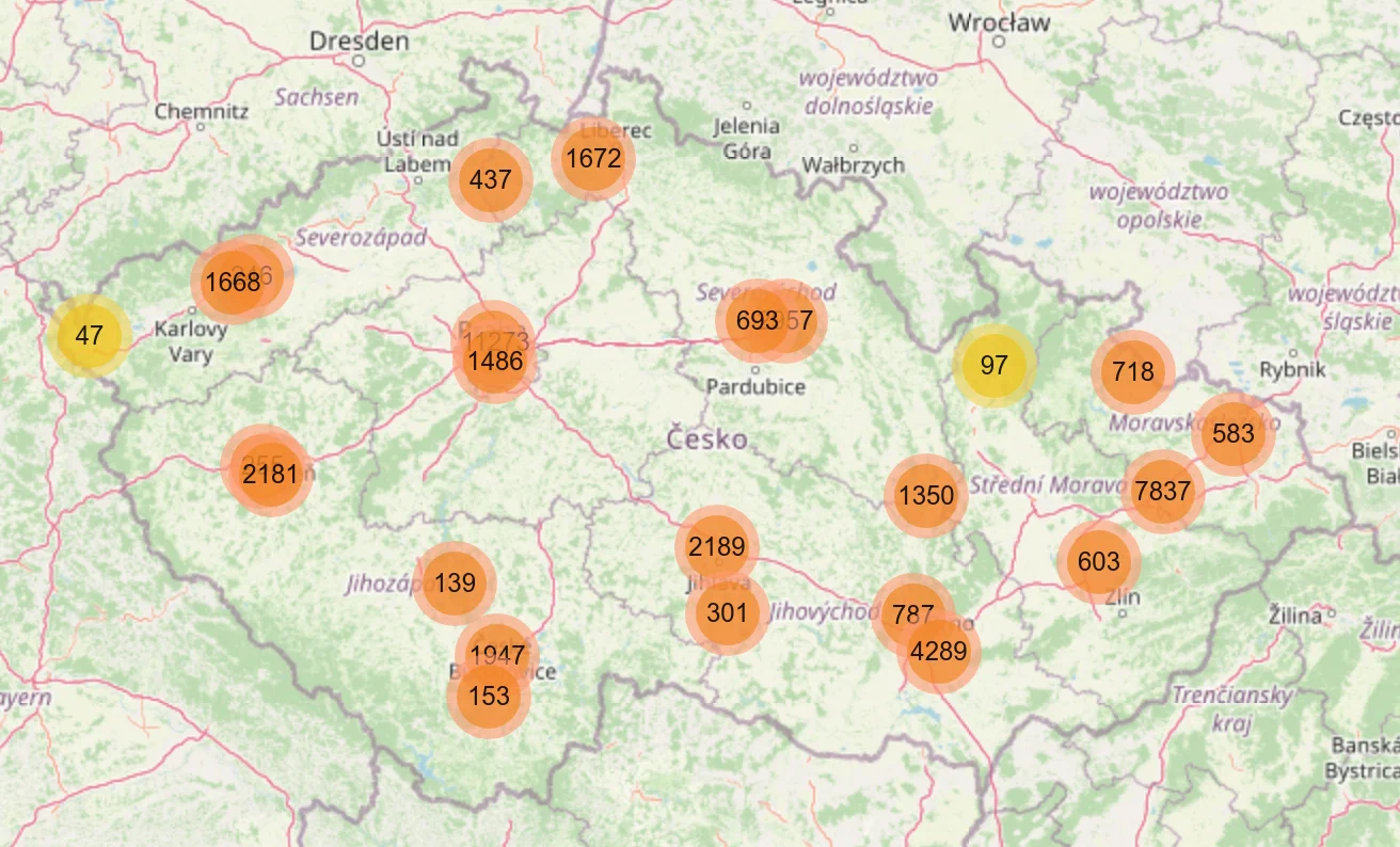
To make it easy for your computer, we are displaying the screenshot of the map here

Neither the map nor the online research we did helped us to fill in the missing data. Given that department_ids and contractual_specialty_ids are essential for the task, we will have to drop the clinics that are missing them. Room for improvement lies within properly filling that data.

Ambulance Stations

ambulance_stations = pd.read_csv('./table_ZZS.csv')
ambulance_stations.head()

	intern_subj_id	name	village	street	number	zip	WGS84_E	WGS84_N	company_id	department_id
0	92	Zdravotnická záchranná služba hl .m. Prahy	Praha	28. pluku	1393	10100	14.464515	50.070763	5001000	5001109
1	92	Zdravotnická záchranná služba hl .m. Prahy	Praha	Chelčického	842	13000	14.458671	50.083906	5001000	5001113
2	92	Zdravotnická záchranná služba hl .m. Prahy	Praha	Dukelských hrdinů	342	17000	14.431312	50.096500	5001000	5001102
3	92	Zdravotnická záchranná služba hl .m. Prahy	Praha	Generála Janouška	902	19800	14.572139	50.106939	5001000	5001110
4	92	Zdravotnická záchranná služba hl .m. Prahy	Praha	Heyrovského náměstí	1987	16200	14.340193	50.086547	5001000	5001104

ambulance_stations.info()

<class 'pandas.core.frame.DataFrame'>
RangeIndex: 332 entries, 0 to 331
Data columns (total 10 columns):
 #   Column          Non-Null Count  Dtype  
---  ------          --------------  -----  
 0   intern_subj_id  332 non-null    int64  
 1   name            332 non-null    object 
 2   village         332 non-null    object 
 3   street          307 non-null    object 
 4   number          332 non-null    int64  
 5   zip             332 non-null    int64  
 6   WGS84_E         332 non-null    float64
 7   WGS84_N         332 non-null    float64
 8   company_id      332 non-null    int64  
 9   department_id   332 non-null    int64  
dtypes: float64(2), int64(5), object(3)
memory usage: 26.1+ KB

Some ambulance stations are missing streets, but that’s OK since we can calculate driving distances based on lat,lon.

Pre-processing

Since we were unable to fill in the missing clinics contractual_specialty_ids and department_ids, let’s drop all of the clinics that are missing them.

clinics.dropna(subset=['contractual_specialty_id'], inplace=True)
clinics.reset_index(drop=True, inplace=True)
len(clinics.index), clinics['contractual_specialty_id'].nunique()

(38081, 273)

Ambulance stations and clinic departments have the same structure and, for the purpose of the task, it would make sense to think of ambulance stations as clinics of a special type. To do this, we introduce a special type 'AST', assign it to the ambulance stations, and concatenate them with the clinics.

ambulance_stations['contractual_specialty_id'] = 'AST'
orgs = clinics.append(ambulance_stations, ignore_index=True)
len(orgs.index), orgs['contractual_specialty_id'].nunique()

(38413, 274)

We copy the coordinates to a new location column in (lat, lon) format to make working with them more convenient.

users['location'] = list(zip(users['WGS84_N'], users['WGS84_E']))
orgs['location'] = list(zip(orgs['WGS84_N'], orgs['WGS84_E']))

As we saw during the clinic analysis, most of the clinic departments share locations and can be uniquely identified by a combination of contractual_specialty_id and department_id. Let’s create a table of parent organizations with a row for each set of clinics that share their location.

orgs['specialty_department'] = list(zip(
    orgs['contractual_specialty_id'],
    orgs['department_id']
))
parent_orgs = orgs.groupby('location').agg({
    'contractual_specialty_id': set,
    'specialty_department': list,
    'location': 'first'
})
print(len(parent_orgs.index))
parent_orgs.head()

location	contractual_specialty_id	specialty_department	location
(48.614218906, 14.311215042)	{014}	[(014, 33866100.0), (014, 33866200.0)]	(48.614218906, 14.311215042)
(48.617204511, 14.313272811)	{AST, 709, 799}	[(709, 32091122.0), (799, 32091822.0), (AST, 3…	(48.617204511, 14.313272811)
(48.617317188, 14.310456114)	{001, 902}	[(001, 33709000.0), (902, 33850100.0)]	(48.617317188, 14.310456114)
(48.618122407, 14.309835495)	{903}	[(903, 33721000.0)]	(48.618122407, 14.309835495)
(48.618840446, 14.30797346)	{014}	[(014, 33701000.0)]	(48.618840446, 14.30797346)

This leaves us with 10,797 of the “actual” clinics that we will be computing routes to. We’ve stored a set of contractual_specialty_ids to a conctractual_specialty_id column to speed up the check for matching specialty ids.

From the start, we’ve aimed for maximum precision. The most precise way to solve the task would be to compute distances for each user individually, so we’ve implemented this straightforward solution first to identify the slowest part of the process and work from there.

It turned out that the slowest part is, not surprisingly, routing and that we will have to optimize it. Clustering users, and maybe, clinics, seemed like a good idea to explore.

The most difficult part of the task is to find a performant solution without sacrificing much of the precision.

Maps

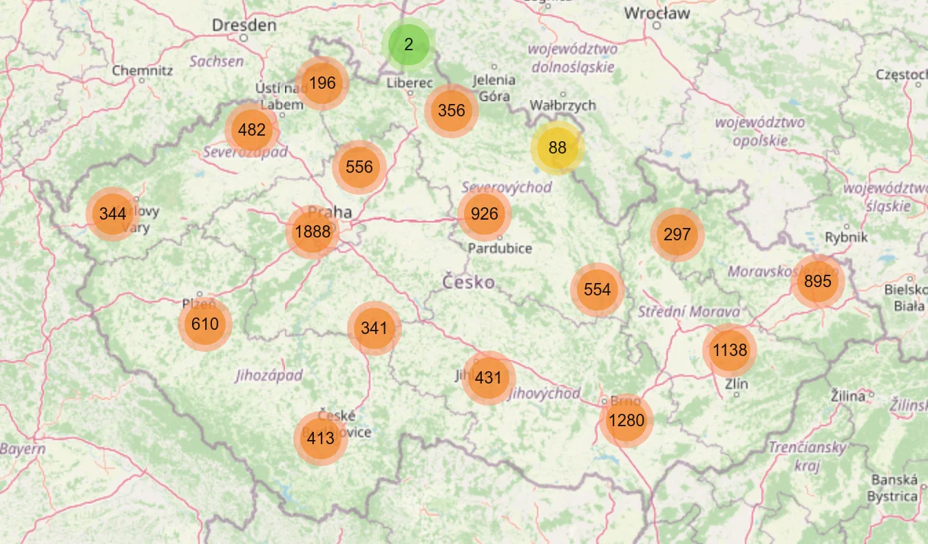
Let’s return to the data exploration and plot parent_orgs and users.

orgs_map = ll.Map(center=CENTER_OF_CZECHIA, zoom=7, min_zoom=7, max_zoom=19)
orgs_map.add_control(ll.FullScreenControl())
orgs_map.add_layer(ll.MarkerCluster(markers=[
    ll.Marker(location=org['location']) for _, org in parent_orgs.iterrows()
]))
orgs_map

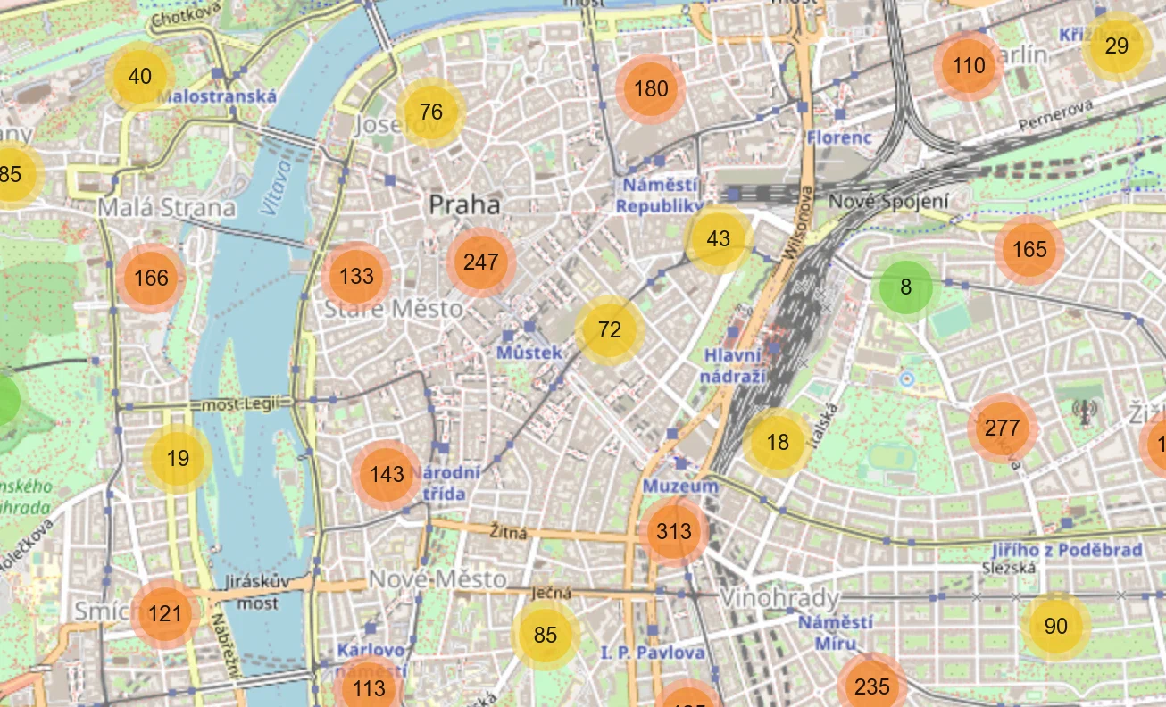
users_map = ll.Map(center=CENTER_OF_CZECHIA, zoom=7, min_zoom=7, max_zoom=19)
users_map.add_control(ll.FullScreenControl())
users_map.add_layer(ll.MarkerCluster(markers=[
    ll.Marker(location=org['location']) for _, org in users[users['village'] == 'Praha'].iterrows()
]))
users_map

It’s interesting to take a look at the Voronoi regions of different clinic types. They can provide us a way to query for candidates.

In mathematics, a Voronoi diagram is a partition of a plane into regions close to each of a given set of objects. In the simplest case, these objects are just finitely many points in the plane (called seeds, sites, or generators). For each seed there is a corresponding region, called Voronoi cells, consisting of all points of the plane closer to that seed than to any other.
— Voronoi diagram - Wikipedia

To compute the regions, we will use the geovoronoi library. Since it uses shapely polygons, we will import the shapely module too. We will also import geopandas to simplify manipulations with the locations in our pandas’ tables and convert them to shapely format.

import geopandas as gpd
import geovoronoi
import shapely.geometry as shg

Then, let’s convert our users and parent_orgs to geo-aware users_geo and orgs_geo tables.

users_geo = gpd.GeoDataFrame(
    users,
    crs='EPSG:4326',
    geometry=gpd.points_from_xy(users['WGS84_E'], users['WGS84_N'])
)

org_locs = list(zip(*parent_orgs['location']))
orgs_geo = gpd.GeoDataFrame(
    parent_orgs,
    crs='EPSG:4326',
    geometry=gpd.points_from_xy(org_locs[1], org_locs[0])
)

We will also need a helper method to convert shapely polygons to leaflet format:

def polygon_to_ll(polygon):
    if isinstance(polygon, shg.Point):
        return [(polygon.y, polygon.x)]
    if isinstance(polygon, shg.LineString):
        return [(point[1], point[0]) for point in polygon.coords]
    return [(point[1], point[0]) for point in polygon.exterior.coords]

And a simple method to plot regions for an org type:

# a polygon encompassing all of the users
all_users = users_geo.unary_union.convex_hull

def plot_voronoi_regions_for_org_by_type(org_type):
    region_polys, region_pts = geovoronoi.voronoi_regions_from_coords(
        orgs_geo[orgs_geo['contractual_specialty_id'] & {org_type}]['geometry'].tolist(),
        all_users
    )

    voronoi_map = ll.Map(center=CENTER_OF_CZECHIA, zoom=7, min_zoom=7, max_zoom=19)
    voronoi_map.add_control(ll.FullScreenControl())
    voronoi_map.add_layer(ll.Polygon(
        locations=[polygon_to_ll(poly) for poly in region_polys.values()],
        color="green",
        fill_color="green"
    ))
    return voronoi_map

We will plot Voronoi regions for one of the most common types of clinics and one of the rarest.

plot_voronoi_regions_for_org_by_type('014')

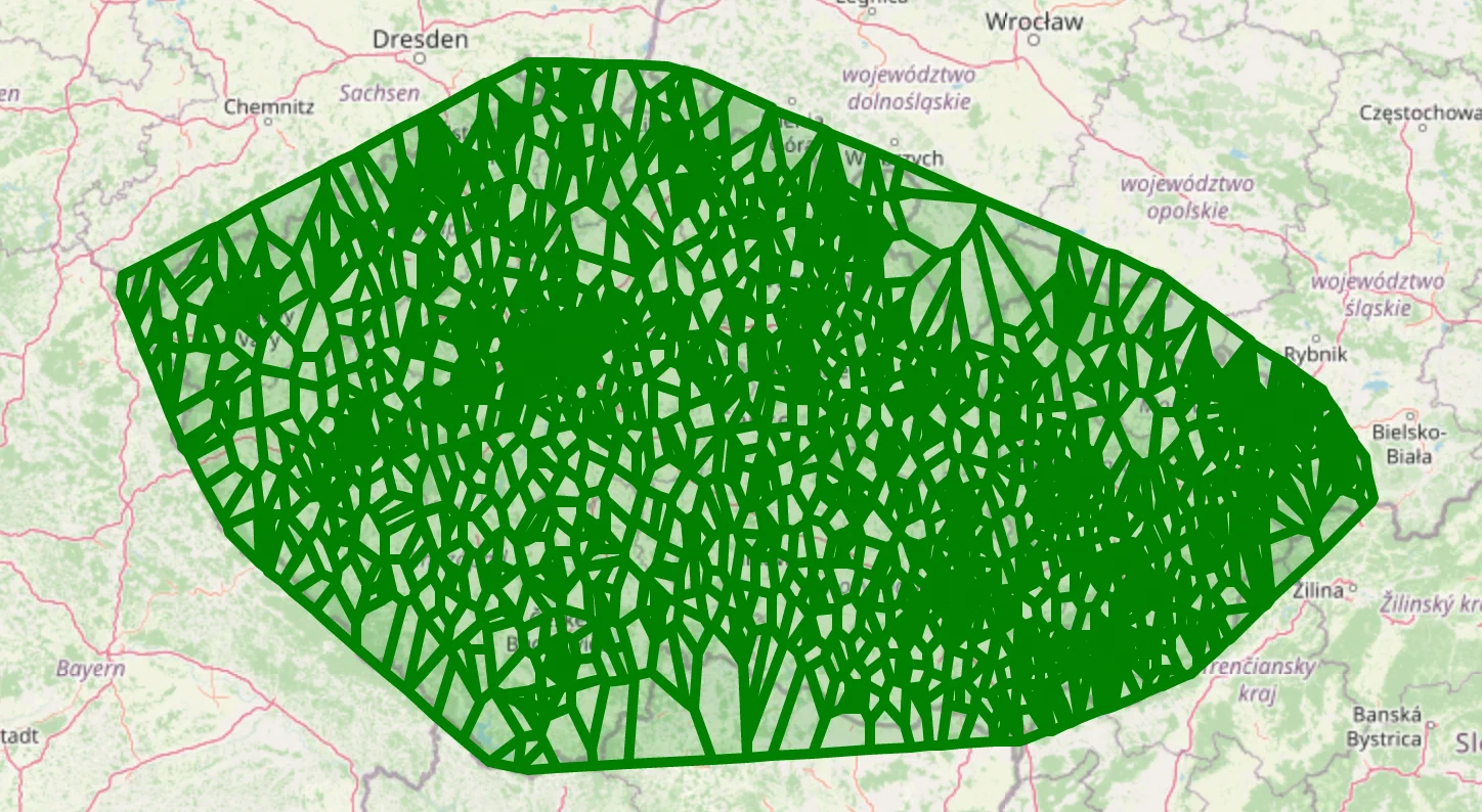
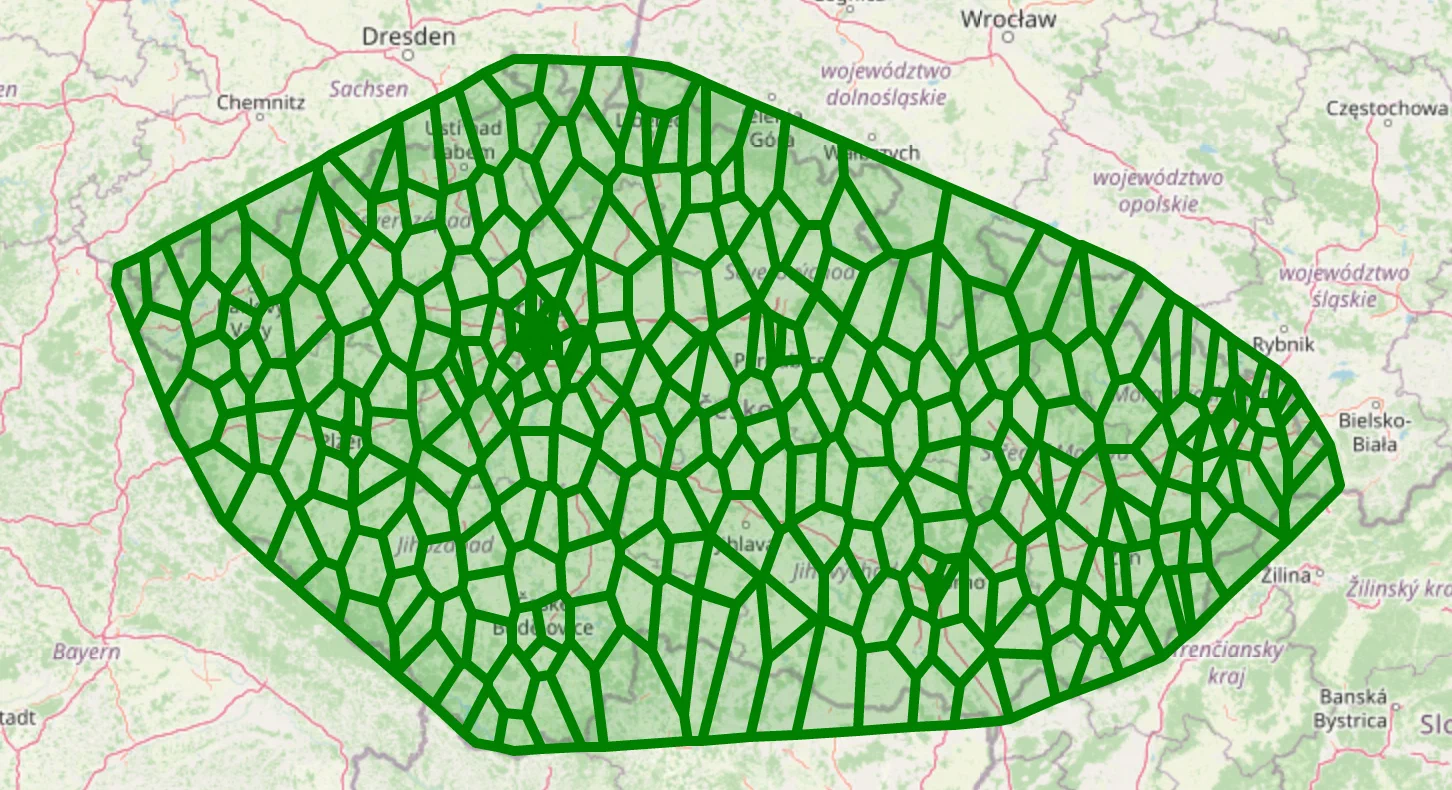
plot_voronoi_regions_for_org_by_type('504')

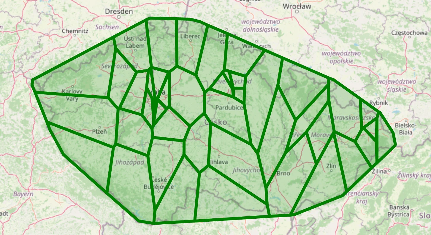
As you can see, some clinics have very sparse coverage; if they represent an essential specialty, there needs to be more of them.

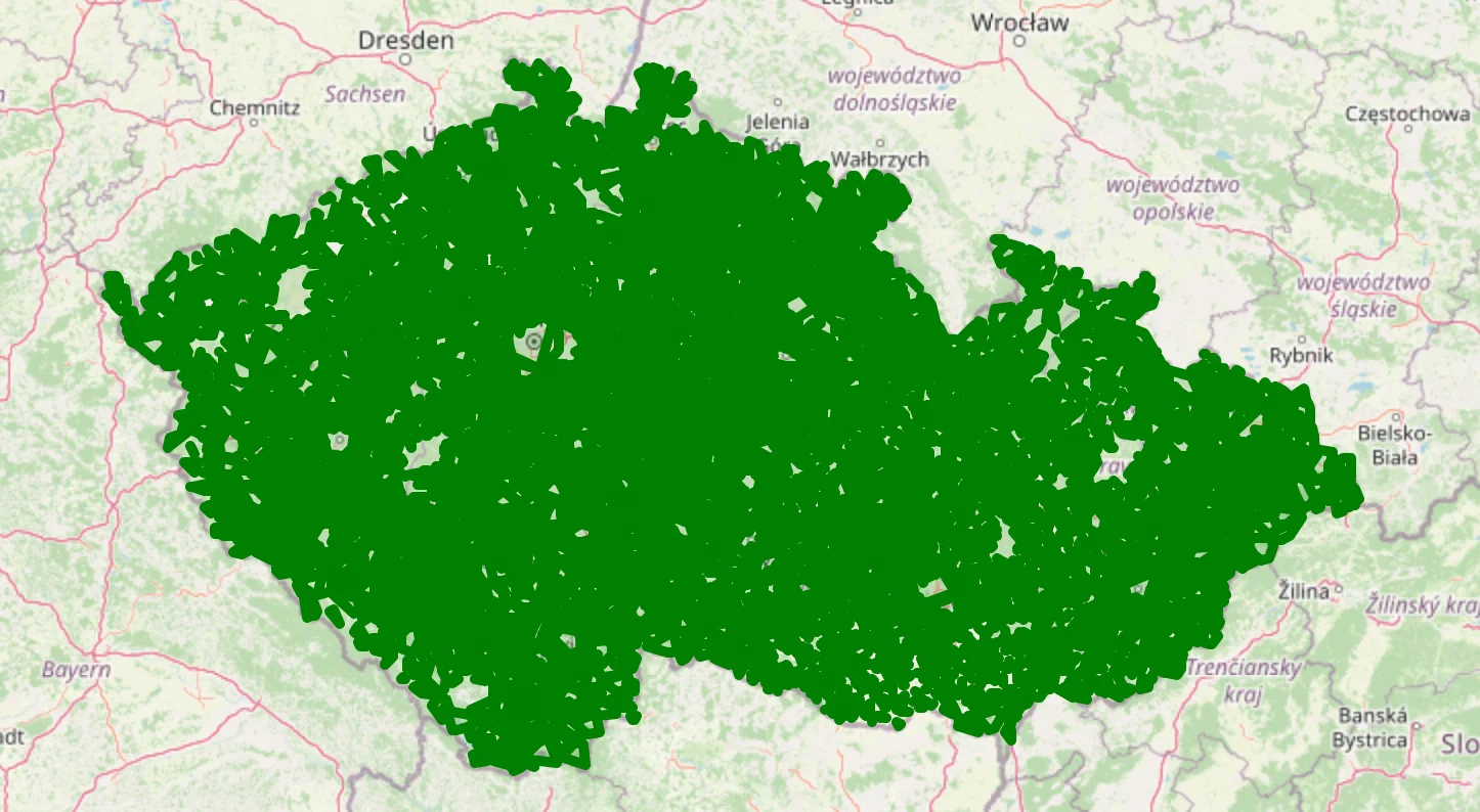
plot_voronoi_regions_for_org_by_type('AST')

These Voronoi regions provide better insight into the clinic density and distribution.

Clusters

Next up is clustering. We decided to cluster users by distance using village information to speed up the clustering.

Utils

Vincenty’s formulae offer one of the most commonly adopted methods to compute the geodesic distance. It’s pretty precise but comparably slow in comparison to the great circle distance computation. To compute the latter, we will use the haversine formula. The haversine formula is much simpler, and therefore, much faster. Let’s see by how much.

We will use geographiclib’s implementation of Vincenty’s formula. It’s a great library of various geodesic algorithm implementations. For the haversine formula, we will use the python haversine library.

from geographiclib.geodesic import Geodesic as geo
import haversine

point_a = (50.088036196500006, 15.820675680125)
point_b = (50.036845777, 15.774167073)

%timeit geo.WGS84.Inverse(*point_a, *point_b)

76.7 µs ± 1.49 µs per loop (mean ± std. dev. of 7 runs, 10000 loops each)

%timeit haversine.haversine(point_a, point_b, haversine.Unit.METERS)

1.31 µs ± 10.8 ns per loop (mean ± std. dev. of 7 runs, 1000000 loops each)

geo.WGS84.Inverse(*point_a, *point_b)['s12'], haversine.haversine(point_a, point_b, haversine.Unit.METERS)

(6596.260963017945, 6589.524077151891)

The difference in performance is staggering when the error margin is negligible. Given that we will only be using this distance for approximations, and both distances are very optimistic approximations of the driving distance, we will stick to the haversine distance going forward.

Before we move on, let’s import the progress bar. Things we do from this moment on will take much more time to compute, and it’s nice to monitor the progress.

from fastprogress.fastprogress import progress_bar

Below is the method that we will use to compute and plot the clusters.

def plot_user_clusters_by(key_fn, radius_m=10_000):
    clusters = {}

    for i, user in progress_bar(users_geo.iterrows(), total=len(users_geo.index)):
        key = key_fn(user)
        user_loc = user['location']
        if key not in clusters:
            clusters[key] = [[(i, user_loc)]]
        else:
            found_cluster = False
            for cluster in clusters[key]:
                first_user_location = cluster[0][1]
                distance = haversine.haversine(
                    first_user_location,
                    user['location'],
                    haversine.Unit.METERS
                )
                if distance < radius_m:
                    found_cluster = True
                    cluster.append((i, user_loc))
                    break
            if not found_cluster:
                clusters[key].append([(i, user_loc)])
                
    cluster_geometries = [
        shg.MultiPoint([(point[1][1], point[1][0]) for point in cluster])
        for cluster_group in clusters.values() for cluster in cluster_group
    ]
    print(f'found {len(cluster_geometries)} clusters')
    
    cluster_map = ll.Map(center=CENTER_OF_CZECHIA, zoom=7, min_zoom=7, max_zoom=19)
    cluster_map.add_control(ll.FullScreenControl())
    cluster_map.add_layer(ll.Polygon(
        locations=[polygon_to_ll(cluster.convex_hull) for cluster in cluster_geometries],
        color="green",
        fill_color="green"
    ))
    return cluster_map,cluster_geometries,clusters

Visualizations

First, we will compute the clusters by user villages.

key_fn = lambda user: user['village']
cluster_map, cluster_geometries, clusters = plot_user_clusters_by(key_fn)
cluster_map

found 6285 clusters

6,285 clusters is a good amount, but the clusters are quite large. Let’s compute clusters based on the user village_parts.

key_fn = lambda user: f'{user["village"]}_{user["village_part"]}'
cluster_map, cluster_geometries, clusters = plot_user_clusters_by(key_fn)
cluster_map

found 14728 clusters

15k is a good amount of clusters in terms of the number of requests we can issue to the Azure API, but the clusters are still quite large. Let’s explore 500m radius clusters.

cluser_map, cluster_geometries, clusters = plot_user_clusters_by(
    lambda user: f'{user["village"]}_{user["village_part"]}',
    radius_m=500
)
cluster_map

found 47199 clusters

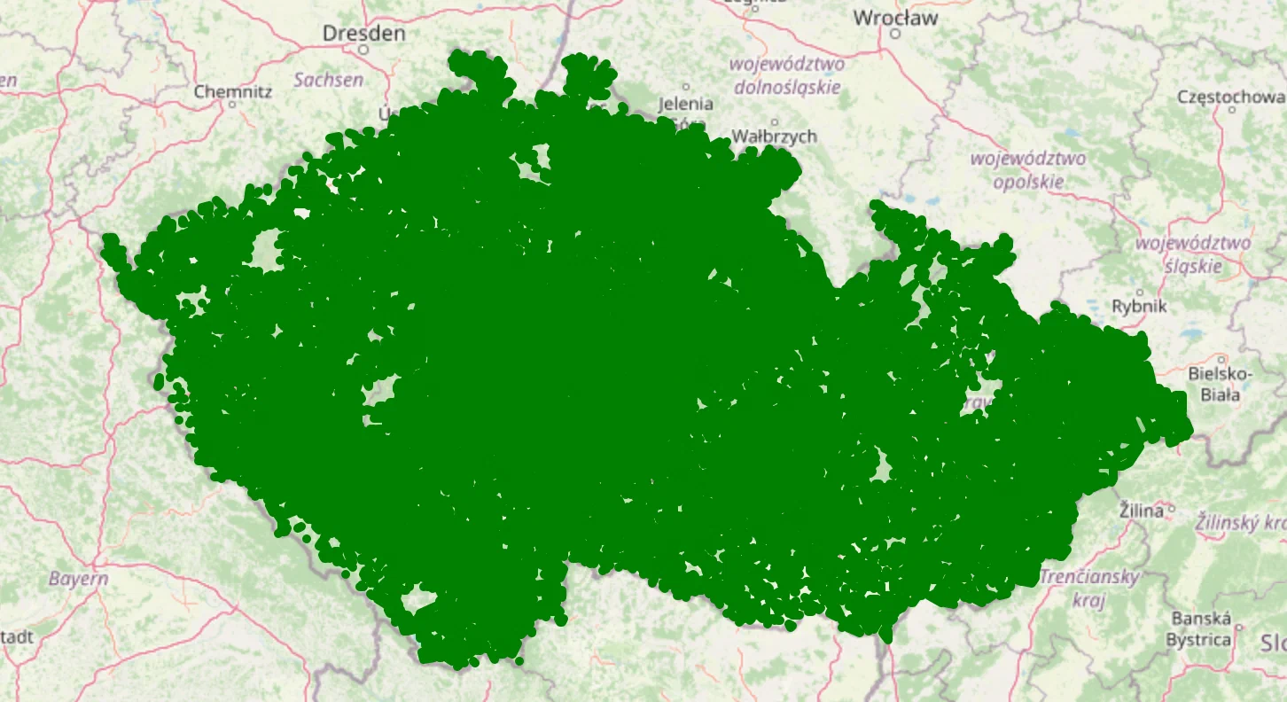
These 47k clusters seem like the way to go for an efficient and precise solution.

Routing

With $200USD in MS Azure credit, we can run only 40k queries against the routing API if we want to send more than 50 of them per second. And with 47k clusters, we would definitely need to send > 40k requests.

To not sacrifice the precision and to iterate quickly, we set up a local instance of the open street routing machine. What follows is the code we used to send routing requests to it.

import requests

OSRM_URI = 'http://127.0.0.1:5000'
MAX_ATTEMPTS = 7

osrm_client = requests.Session()


def request(url, attempt=1):
    try:
        response = osrm_client.get(url)
        response.raise_for_status()
        return response
    except Exception as e:
        if attempt > MAX_ATTEMPTS:
            raise e
        return request(url, attempt + 1)

    
def get_route(lat1, lon1, lat2, lon2):
    url = f'{OSRM_URI}/route/v1/driving/{lon1},{lat1};{lon2},{lat2}?continue_straight=false'
    try:
        response = request(url)
        route = response.json()['routes'][0]
    except:
        print('[get_route] err', url)
        return float('inf'), float('inf'), ''
    return route['distance'], route['duration'] / 60, route['geometry']

Let’s make sure that it works and get some sense of the performance.

get_route(50.077033696848886, 14.440035214801874, 50.070578695594314, 14.494946221573803)

(5248, 7.403333333333333, 'evspH{icwAv@aK@{RkGsmDzIalBgBgt@b_@yCpBvL|ExKQtC')

%timeit get_route(50.077033696848886, 14.440035214801874, 50.070578695594314, 14.494946221573803)

1.86 ms ± 109 µs per loop (mean ± std. dev. of 7 runs, 100 loops each)

Solution

The solution is quite straightforward from that point on. But before we move on, let’s import numpy.

import numpy as np

We will need a ~~fast~~vectorized method for the haversine distance computation.

def sort_data_haversine(points, data):
    distances = haversine.haversine_vector(
        data['location'].tolist(),
        points['location'].tolist(),
        unit=haversine.Unit.METERS,
        comb=True
    )
    return np.argsort(distances), distances

index, distances = sort_data_haversine(users[:100], parent_orgs)
index, distances

(array([[4989, 4992, 4911, ..., 3372, 3375, 3254],
        [4989, 4992, 4911, ..., 3372, 3375, 3254],
        [4989, 4992, 4911, ..., 3372, 3375, 3254],
        ...,
        [4743, 4803, 4799, ..., 3372, 3375, 3254],
        [3362, 3146, 3320, ..., 3807, 3375, 3254],
        [4827, 4803, 4799, ..., 3372, 3375, 3254]]),
 array([[133852.36820813, 133508.21170191, 133514.27117984, ...,
         138680.78292498, 134174.19127045, 140410.66063062],
        [133888.2414056 , 133543.99335324, 133550.20998843, ...,
         138626.18005503, 134154.00442703, 140355.03132468],
        [134038.57941885, 133694.36931002, 133700.5206838 , ...,
         138486.67124833, 133999.0278078 , 140216.3122906 ],
        ...,
        [132402.65539979, 132050.23378999, 132072.18742985, ...,
         138917.42961128, 137858.06810736, 140528.10016674],
        [109703.4194728 , 109348.16998337, 109376.71678102, ...,
         161563.91234588, 160672.22237329, 163126.36755815],
        [134407.99756303, 134053.95329282, 134079.57745343, ...,
         136852.37604113, 136692.76736826, 138434.94454964]]))

%timeit sort_data_haversine(users[:100], parent_orgs)

75.7 ms ± 63.3 µs per loop (mean ± std. dev. of 7 runs, 10 loops each)

75ms to compute 100*11k distances is pretty good.

ORG_TYPES = set(orgs['contractual_specialty_id'].unique())
len(ORG_TYPES)

Next, we will create a method to find solutions for each of the clusters. To be performant, we look for all types of clinics in a single pass over a sorted list of candidates. It’s hard to vectorize the method, so we run it in multiple threads.

Notice that the solution incorporates our knowledge that there are some clinics of the same type that share the exact location. When we encounter this, we randomly distribute users between such clinics to provide better coverage.

import concurrent.futures
import random

pool = concurrent.futures.ProcessPoolExecutor(max_workers=10)

def find_closest_orgs_for_point(point, index, distances):
    org_types_left = ORG_TYPES.copy()
    result = {}
    for i in index:
        if not org_types_left:
            break
        parent_org = parent_orgs.iloc[i]
        haversine_distance = distances[i]
        route = None
        for specialty_department in (sd for sd in parent_org['specialty_department'] if sd[0] in org_types_left):
            specialty = specialty_department[0]
            best_route = result.get(specialty, ((float('inf'),),))[0]
            if haversine_distance > best_route[0]:
                org_types_left.remove(specialty)
                continue
            if not route:
                route = get_route(*point['location'], *parent_org['location'])
            if (route[0] < best_route[0]) or (route[0] == best_route[0] and random.random() < .5):
                result[specialty] = (route, specialty_department, parent_org['location'])
    return result


def _wrapper(args):
    return find_closest_orgs_for_point(*args)


def find_closest(points, orgs: pd.DataFrame):
    index, distances = sort_data_haversine(points, parent_orgs)
    return list(pool.map(_wrapper, [
        (points.iloc[i], index[i], distances[i]) for i in range(len(index))
    ]))

users_res = find_closest(users[:1], parent_orgs)
list(users_res[0].values())[:5]

[((3473.6,
   5.298333333333333,
   '_d`oHyxjwAK{@g@a@qA|BeFvCYCSs@pCkGjBcIJsEw@cKZgGz@qAbCkAv@uBXg_@i@iFaCoFiBkJ{GaPg@aDiBq{@cCyVo@iL?qJv@gGZDAj@'),
  ('014', 20216001.0),
  (49.816801772, 14.517831226)),
 ((3473.6,
   5.298333333333333,
   '_d`oHyxjwAK{@g@a@qA|BeFvCYCSs@pCkGjBcIJsEw@cKZgGz@qAbCkAv@uBXg_@i@iFaCoFiBkJ{GaPg@aDiBq{@cCyVo@iL?qJv@gGZDAj@'),
  ('002', 20412001.0),
  (49.816801772, 14.517831226)),
 ((3476.6,
   5.341666666666667,
   '_d`oHyxjwAK{@g@a@qA|BeFvCYCSs@pCkGjBcIJsEw@cKZgGz@qAbCkAv@uBXg_@i@iFaCoFiBkJ{GaPg@aDiBq{@cCyVo@iLAaJx@wG}@R'),
  ('902', 20721001.0),
  (49.817220095, 14.517841305)),
 ((16488.6,
   28.763333333333332,
   '_d`oHyxjwAFrXf@|@rAIhBkKx@w@tDrC~GnVpOkD|EkCSzSqBpF`BzM~BtB~Kh`@|JzQvCn@nBkAwJt\\oJ|LMnAh@xC~EnE|A|DfKxY`ArG[hEuCzH~@lLkBnDwBzAuEmA}AlHwN|BoMsNoBMiAzAIdDzCfNYpGyHfI{JpC}HtFkF\\_VuDuR|@gEsCiCiH~@gM[sC_LeEcDpHm@|UXfH_@bBkExDQtCz@x@jGQxFzBfKfAbDfCvBpEEtCcDdObDvLAh\\t@xOxGtc@xLjd@l@hFXwChFaAbH}HvBqMzE{GdC_H`De@zAjHxC`AfLaGRwHnAoG}AgELmAnDb@`CpF|NdLvS?rCuIxEwEZwR{AiKp@eCh@g_@uC{WaG_V'),
  ('709', 22107293.0),
  (49.800521335, 14.42696598)),
 ((16488.6,
   28.763333333333332,
   '_d`oHyxjwAFrXf@|@rAIhBkKx@w@tDrC~GnVpOkD|EkCSzSqBpF`BzM~BtB~Kh`@|JzQvCn@nBkAwJt\\oJ|LMnAh@xC~EnE|A|DfKxY`ArG[hEuCzH~@lLkBnDwBzAuEmA}AlHwN|BoMsNoBMiAzAIdDzCfNYpGyHfI{JpC}HtFkF\\_VuDuR|@gEsCiCiH~@gM[sC_LeEcDpHm@|UXfH_@bBkExDQtCz@x@jGQxFzBfKfAbDfCvBpEEtCcDdObDvLAh\\t@xOxGtc@xLjd@l@hFXwChFaAbH}HvBqMzE{GdC_H`De@zAjHxC`AfLaGRwHnAoG}AgELmAnDb@`CpF|NdLvS?rCuIxEwEZwR{AiKp@eCh@g_@uC{WaG_V'),
  ('799', 22107493.0),
  (49.800521335, 14.42696598))]

%timeit -n1 -r1 find_closest(users[:100], parent_orgs)

33.2 s ± 0 ns per loop (mean ± std. dev. of 1 run, 1 loop each)

Our implementation can find the solution for 100 users in 33 seconds. We are ready to run it on user clusters, and before we do, we have to compute the centroids of the clusters.

clusters_flat = [cluster for cluster_group in clusters.values() for cluster in cluster_group]
clusters_restructured = [list(zip(*cluster)) for cluster in clusters_flat]
clusters_geo = gpd.GeoDataFrame(
    clusters_restructured,
    crs='EPSG:4326',
    columns=['users', 'locations'],
    geometry=cluster_geometries
)
clusters_geo.head()

	users	locations	geometry
0	(0, 1, 2, 3, 6, 7, 8, 9, 10, 12, 14, 15, 16, 1…	((49.813014079, 14.478449504), (49.813251371, …	MULTIPOINT (14.47845 49.81301, 14.47990 49.813…
1	(4,)	((49.814779761, 14.469590894),)	MULTIPOINT (14.46959 49.81478)
2	(13,)	((49.810529999, 14.460041926),)	MULTIPOINT (14.46004 49.81053)
3	(11629, 11650, 11659, 11673, 11724, 11729, 117…	((49.98905532, 14.203808164), (49.993207327, 1…	MULTIPOINT (14.20381 49.98906, 14.20444 49.993…
4	(11642, 11653, 11685, 11699, 11714, 11726, 117…	((49.993481837, 14.21378659), (49.993255048, 1…	MULTIPOINT (14.21379 49.99348, 14.21489 49.993…

cluster_centroids = clusters_geo.centroid.to_frame()
cluster_centroids['location'] = cluster_centroids.applymap(lambda centroid: (centroid.y, centroid.x))
cluster_centroids.head()

<ipython-input-56-c0091e7f21d9>:1: UserWarning: Geometry is in a geographic CRS. Results from 'centroid' are likely incorrect. Use 'GeoSeries.to_crs()' to re-project geometries to a projected CRS before this operation.

  cluster_centroids = clusters_geo.centroid.to_frame()

	0	location
0	POINT (14.47861 49.81427)	(49.81426659066666, 14.478608245733335)
1	POINT (14.46959 49.81478)	(49.814779761, 14.469590894)
2	POINT (14.46004 49.81053)	(49.810529999, 14.460041926)
3	POINT (14.20518 49.99149)	(49.99148887917857, 14.205177951250004)
4	POINT (14.21365 49.99239)	(49.99238546947369, 14.21365326868421)

Once they are computed, we are ready to process all of the clusters.

BATCH_SIZE = 1000

cluster_results = []

total_iterations = np.ceil(len(cluster_centroids.index) / BATCH_SIZE)

for i in progress_bar(range(0, len(cluster_centroids.index), BATCH_SIZE), total=total_iterations):
    batch_results = find_closest(cluster_centroids[i:i+BATCH_SIZE], parent_orgs)
    cluster_results += batch_results

Running the solution on 47k clusters took 3 hours and 40 minutes, a time we are quite happy with.

The last thing left is writing the output CSV. Before we proceed, let’s remind ourselves how it should look like.

OUTPUT_COLUMNS

['policyholder_num',
 'contractual_specialty_id',
 'pzs_department_id',
 'km_to_pzs',
 'min_to_pzs',
 'zzs_department_id',
 'km_to_zzs',
 'min_to_zzs']

Because we really care about precision, we will adjust distance and driving times for each user based on the ratio between user⇔clinic and cluster centroid⇔clinic straight line distances.

import csv

M_IN_KM = 1000
SPEED = 833  # meters per hour (50kmh), used only when centroid2org distance is 0 (rare)


def adjust_route(route, user_location, centroid_location, org_location):
    centroid2org_distance = haversine.haversine(
        centroid_location,
        org_location,
        haversine.Unit.METERS
    )
    user2org_distance = haversine.haversine(
        user_location,
        org_location,
        haversine.Unit.METERS
    )
    if centroid2org_distance == 0:
        return user2org_distance, user2org_distance / SPEED, route[2]
    ratio = user2org_distance / centroid2org_distance
    return route[0] * ratio, route[1] * ratio, route[2]


with open('./output.csv', 'w') as file:
    writer = csv.writer(file)
    writer.writerow(OUTPUT_COLUMNS)
    
    for cluster_i, cluster in progress_bar(clusters_geo.iterrows(), total=len(clusters_geo.index)):
        cluster_rows = []
        ast_route, ast_org, ast_location = cluster_results[cluster_i]['AST']
        centroid_location = cluster_centroids.iloc[cluster_i]['location']
        for user_i in cluster['users']:
            user = users.iloc[user_i]
            user_loc = user['location']
            adj_ast_route = adjust_route(
                ast_route,
                user_loc,
                centroid_location,
                ast_location
            )
            for cluster_result in cluster_results[cluster_i].values():
                route, clinic, clinic_location = cluster_result
                if clinic[0] == 'AST':
                    continue
                adj_route = adjust_route(
                    route,
                    user_loc,
                    centroid_location,
                    clinic_location
                )
                cluster_rows.append([
                    user['policyholder_num'],
                    clinic[0],
                    f'{int(clinic[1]):08d}',
                    adj_route[0] / M_IN_KM,
                    adj_route[1],
                    f'{int(ast_org[1]):08d}',
                    adj_ast_route[0] / M_IN_KM,
                    adj_ast_route[1],
                ])
        writer.writerows(cluster_rows)

As you can see, we came up with an elegant, efficient, and precise solution by thoroughly analyzing the data, clustering the users, setting up the local routing machine, vectorizing and parallelizing the computations, and approximating final driving distances and times for each of the users individually.

Result visualization

Let us conclude by plotting the results for a few clusters.

import polyline

CLUSTER_COLORS = ['green', 'red', 'orange']

routes_map = ll.Map(center=CENTER_OF_CZECHIA, zoom=7, min_zoom=7, max_zoom=19)
routes_map.add_control(ll.FullScreenControl())

for i in range(len(CLUSTER_COLORS)):
    cluster_color = CLUSTER_COLORS[i]
    cluster_result = cluster_results[i * 10000]
    for j, specialty_result in enumerate(cluster_result.items()):
        _, result = specialty_result
        route = polyline.decode(result[0][2])
        routes_map.add_layer(ll.Polyline(
            locations=route,
            color=cluster_color,
            fill=False
        ))
        routes_map.add_layer(ll.Marker(
            location=route[-1],
            icon=ll.AwesomeIcon(name='hospital-o'),
            draggable=False
        ))
        if j == 0:
            routes_map.add_layer(ll.Marker(
                location=route[0],
                icon=ll.AwesomeIcon(name='users', marker_color=cluster_color),
                draggable=False
            ))
        
routes_map

This map is interactive, and results for each of the clusters are color-coded; feel free to explore it. I hope that you’ve enjoyed this article! If you have any thoughts about it, please, reach out to me on Twitter.

I want to end by saying thank you to the ML Prague Conference, SAS, and all other sponsors for the hackathon! I had a lot of fun and am already looking forward to next year! :)